Introduction

(Hoffman & Johnson, 2016) proposed an elegant decomposition of the evidence lower bound, or ELBO, objective commonly used to train unsupervised latent-variable models characterized by a probabilistic decoder $p(x | z)$ and prior $p(z)$ over latent variable $z$. Such models have the form:

\begin{equation} p_{\theta}(x) = \int p_{\theta} (x | z) p(z) dz \end{equation}

A common way of writing the ELBO objective, for variational approximation $q_{\phi}(z | x)$ to the true posterior $p_{\theta}(z | x)$ is like,

\begin{equation} \label{eq:term-by-term} L({\theta}, {\phi}) = \frac{1}{N} \sum_{n=1}^{N} \mathbb{E}_{q(z_n | x_n)}[\log (p(x_n|z_n))] - KL(q(z_n | x_n) \parallel p(z_n)) \end{equation}

which they call the average term-by-term reconstruction minus the KL divergence to the prior, where $n$ indexes observations. This leads to a natural question: what is the best value for the KL term to take? This can be interpreted as a regularizer that is minimized when $q(z_n | x_n) = p(z_n)$, which encourages maximum use of the code space $z$ by raising the entropy of $q(z)$ to that of the prior. Aside: one of the most common choices for this prior is a multivariate normal: the maximum entropy distribution for a given variance. Now, clearly we do not want this KL term to be exactly zero, as this implies independence between inputs $x_n$ and their codes $z_n$. For examples of this behaviour see the autodecoder in (Alemi et al., 2018), where the generated samples are of high quality, but do not match the class of the input source.

Breaking up the KL divergence term:

\begin{equation} \frac{1}{N} \sum_{n=1}^{N} KL[q(z_n | x_n) \parallel p(z_n)] = D_{KL}(q(z) \parallel p(z)) + \log(N) - \mathbb{E}_{q(z)}[H[q(n|z)]] \end{equation}

Notice that $\log(N) - \mathbb{E}_{q(z)}[H[q(n|z)]]$, looks an awful lot like the mutual information of the form $I(n;z)=H(n)-H(n|z)$, where we’re treating the indices $n$ to the $N$ input samples $X_N$ as a uniform random variable, the maximum entropy distribution for a constraint on the values.

Thus, we have:

\begin{equation} = D_{KL}(q(z) \parallel p(z)) + I(n;z) \end{equation}

where $q(z)$ can safely be made close to the prior without losing modeling power.

Derivation

Using $p(z | n) = p(z)$, $q(z | n) = q(z | x_n)$, $q(n) = p(n) = 1/N$,

\begin{equation} \frac{1}{N} \sum_{n=1}^{N} KL(q(z_n | x_n) \parallel p(z_n)) = \sum_n q(n, z) \log \frac{q(n, z)}{p(n, z)} \end{equation}

$$= \sum_n q(n) q(z|n) \log \frac{q(z) q(n | z)}{p(z) p(n)}$$

Now, splitting up the log

$$= \sum_n q(n) q(z|n) \bigg( \log \frac{q(z)}{p(z)} + \log \frac{q(n | z)}{p(n)} \bigg)$$

\begin{equation} = KL(q(z) \parallel p(z)) + \mathbb{E}_{q(z)}[KL(q(n | z) \parallel p(n))] \end{equation}

With Bayes rule $q(n)q(z|n) = q(z)q(n|z)$, and expanding some terms

$$= KL(q(z) \parallel p(z)) + \sum_n q(z)q(n | z) \bigg( \log \frac{q(n | z)}{p(n)} \bigg)$$ $$= KL(q(z) \parallel p(z)) + \sum_n q(z) \underbrace{q(n | z) \log q(n | z)}_\text{-ve cond. entropy} -\underbrace{\sum_n \log \frac{1}{p(n)}}_\text{entropy of n}$$

Since we have a uniform distribution over $n$, the i.i.d. sample indices, $H(n) = \log N$.

\begin{equation} = KL(q(z) \parallel p(z)) + (\log N - \mathbb{E}_{q(z)}[H(q(n|z))]) \end{equation}

\begin{equation} = KL(q(z) \parallel p(z)) + I(n; z) \end{equation}

Getting back to the original question, we now have clear expressions for the quantities we want to minimize: $KL(q(z) \parallel p(z))$, and maximize: $I(n; z)$.

Now, we have some context for an inequality from (Alemi et al., 2018), where D is distortion—the first term in Eq.\eqref{eq:term-by-term}—and H is $H(X)$, the entropy of the source distribution. R is the rate, the description length or average number of bits transmitted—but not necessarily received.

\begin{equation} H - D \leq I(X; Z) \leq R \end{equation}

Since $KL(q(z) \parallel p(z))$ can be computed analytically for known parametric families, we have a way of estimating $I(X; Z)$ by simply subtracting this term from the ‘‘KL divergence to the prior’’ in Eq.\eqref{eq:term-by-term}, and replacing each $x$ by its index $n$ from the finite training sample.

Sweeping $\beta$ as in the $\beta-VAE$ obtained by breaking up Eq.\eqref{eq:term-by-term}, we obtain a concave rate distortion RD curve. This says that reducing distortion, which in this case can be interpreted as increasing the quality of the reconstructed images, is only possible by increasing the complexity of the representations, and vice versa, reducing the rate is only possible if willing to accept higher distortion.

What are the practical consequences of this trade-off? After all, the cost of bandwidth and computing is at an all time low, can’t we just use arbitrarily high complexity representations to minimize distortion? No, not if we’d like to use the generative model for one of its main functions: to generate novel samples simply by sampling from the prior. See the ‘‘autoencoder’’ example in Fig. 4 b) of (Alemi et al., 2018) where R=156.0 and D=4.8. Thus, we want to be somewhere in between the ‘‘semantic encoder’’ and ‘‘semantic decoder’’ which corresponds to places on the curve where both R and D are changing rapidly. This makes the model capable of both reconstructing natural inputs, and ensures most of the code space maps to plausible samples when sampling from the prior unconditionally.

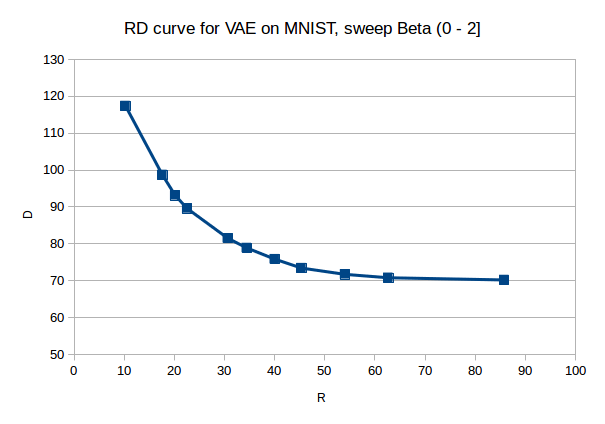
RD curve has units in bits, whereas (Alemi et al., 2018) are in nats, $120$ bits $\times ln2 \approx 83$ nats. (Alemi et al., 2018) obtain $D=80.6$ nats for $R=0$.

References

1. Fixing a Broken ELBO Alemi, Alexander, Poole, Ben, Fischer, Ian, Dillon, Joshua, Saurous, Rif A., and Murphy, Kevin In International Conference on Machine Learning 2018
2. Formal Limitations on the Measurement of Mutual Information McAllester, David, and Stratos, Karl 2018
3. ELBO Surgery: Yet Another Way to Carve up the Variational Evidence Lower Bound Hoffman, Matthew D, and Johnson, Matthew J In NIPS Workshop on Advances in Approximate Bayesian Inference 2016