Link to arXiv Preprint.
Abstract
Batch normalization is often used in an attempt to stabilize and accelerate training in deep neural networks. In many cases it indeed decreases the number of parameter updates required to reduce the training error. However, it also reduces robustness to small input perturbations and noise by double-digit percentages, as we show on five standard datasets. Furthermore, substituting weight decay for batch norm is sufficient to nullify the relationship between adversarial vulnerability and the input dimension. Our work is consistent with a mean-field analysis that found that batch norm causes exploding gradients.
Batch Norm
We briefly review how batch norm modifies the hidden layers’ pre-activations $h$ of a neural network. We use the notation of (Yang, Pennington, Rao, Sohl-Dickstein, & Schoenholz, 2019), where $\alpha$ is the index for a neuron, $l$ for the layer, and $i$ for a mini-batch of $B$ samples from the dataset; $N_l$ denotes the number of neurons in layer $l$, $W^l$ is the matrix of weights and $b^l$ is the vector of biases that parametrize layer $l$. The batch mean is defined as $\mu_\alpha = \frac{1}{B} \sum_i h_{\alpha i}$, and the variance is $\sigma_\alpha^2 = \sqrt{\frac{1}{B} \sum_i {(h_{\alpha i} - \mu_\alpha)}^2 + c}$, where $c$ is a small constant to prevent division by zero. In the batch norm procedure, the mean $\mu_\alpha$ is subtracted from the pre-activation of each neuron $h_{\alpha i}^l$ – consistent with (Ioffe & Szegedy, 2015) –, the result is divided by the standard deviation $\sigma_\alpha$, then scaled and shifted by the learned parameters $\gamma_\alpha$ and $\beta_\alpha$, respectively. This is described in Eqs. \eqref{eq:bn1} and \eqref{eq:bn2}, where a per-unit nonlinearity $\phi$, e.g., ReLU, is applied after the normalization.
\begin{equation} \label{eq:bn1} h_{\alpha i}^l = \gamma_{\alpha} \frac{h_{\alpha i} - \mu_{\alpha}}{\sigma_{\alpha}} + \beta_{\alpha} \end{equation}
\begin{equation} \label{eq:bn2} h_i^l = W^l \phi (h_i^{l - 1}) + b^l \end{equation}
Note that this procedure fixes the first and second moments of all neurons $\alpha$ equally. This suppresses the information contained in these moments. Batch norm induces a nonlocal batch-wise nonlinearity, such that two mini-batches that differ by only a single example will have different representations for each example (Yang, Pennington, Rao, Sohl-Dickstein, & Schoenholz, 2019). This difference is further amplified by stacking batch norm layers. We argue that this information loss and inability to maintain relative distances in the input space reduces adversarial as well as general robustness.
We illustrate this effect by reproducing Fig. 6 of (Yang, Pennington, Rao, Sohl-Dickstein, & Schoenholz, 2019) in the above animation. Two mini-batches that contain the same data points except for one are shown at Layer 0, or input. We propagate the mini-batches through a deep batch-normalized linear network, i.e. with $\phi=id$, and of any practical width. The activations are then projected to their two principal components. This figure reminded me of the Adversarial Spheres dataset for binary classification of concentric spheres on the basis of their differing radii (Gilmer et al., 2018). It turns out that this simple task poses a challenge to the conventional wisdom that batch norm accelerates training and improves generalization; batch norm does the exact opposite in this case, prolonging training by $\approx 50 \times$, increasing sensitivity to the learning rate, and reduces robustness. This is likely why they used the Adam optimizer instead of plain SGD in the original work on Adversarial Spheres, and trained in an online manner for one million steps. The next illustration makes it clear why this is so.
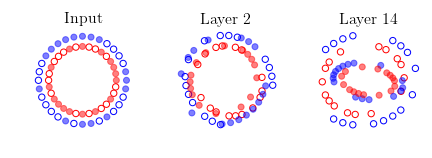
Concentric circles and their representations in a deep linear network with batch norm at initialization. Mini-batch membership is indicated by marker fill and class membership by colour. Each layer is projected to its two principal components. Some samples overlap at Layer 2, and classes are mixed at Layer 14.
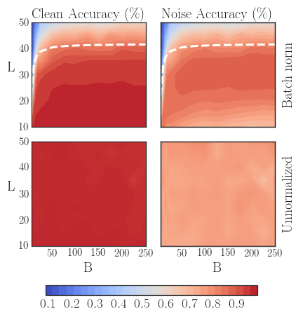
In the next visualization, we repeat the experiment of (Yang, Pennington, Rao, Sohl-Dickstein, & Schoenholz, 2019) by training fully-connected nets of depth $L$ and constant-width ReLU layers for ten epochs by SGD, and learning rate $\eta = 10^{-5} B$ for batch size $B$ on MNIST. The batch norm parameters $\gamma$ and $\beta$ were left as default, momentum was disabled, and $c = 10^{-3}$. Trials were averaged over three random seeds.
It turns out that one can predict the theoretical maximum depth solely as a function of the batch size, due to an – almost paradoxically reliable – gradient explosion due to batch norm. The following function computes this, up to a correction factor since the general form works for any dataset, learning rate, or optimizer. The dashed line shows the theoretical maximum trainable depth in the context of our experiment.
# Thm. 3.10 Yang et al., (2019)
def J_1(c):
    return (1 / np.pi) * (np.sqrt(1 - c**2) + (np.pi - np.arccos(c))*c)

# first derivative of J_1
def J_1_prime(c):
    return - (c / (np.pi * np.sqrt(1 - c**2)))

lambda_G = (1 / (B - 3)) * ((B - 1 + J_1_prime(-1 / (B - 1))) / (1 - J_1(-1 / (B - 1))) - 1)
print(16 * (1 / np.log(lambda_G))) # 16 is a correction factor
References
-
A Mean Field Theory of Batch Normalization In International Conference on Learning Representations 2019
-
Adversarial Spheres In International Conference on Learning Representations Workshop Track 2018
-
Batch Normalization: Accelerating Deep Network Training by Reducing Internal Covariate Shift In International Conference on Machine Learning 2015