Introduction

Intersection over union (IoU) is a common metric for assessing performance in semantic segmentation tasks. In a sense, (IoU) is to segmentation what an F1 score is to classification. Both are non-differentiable, and not normally optimized directly. Optimizing cross entropy loss is a common proxy for these scores, that usually leads to decent performance, provided everything else has been setup correctly, e.g regularization, stopping training at an appropriate time. Divising a pixelwise loss function, such that a deep network performs segmentation, with the mindset of classification and cross-entropy, we get something like this:

Listing 1: TensorFlow pixelwise softmax cross-entropy loss

# logits has original shape [batch_size x img h x img w x FLAGS.num_classes]
logits=tf.reshape(logits, (-1, FLAGS.num_classes))
trn_labels=tf.reshape(trn_labels_batch, [-1])
cross_entropy=tf.nn.sparse_softmax_cross_entropy_with_logits(logits,trn_labels,name='x_ent')
loss=tf.reduce_mean(cross_entropy, name='x_ent_mean')
train_op=tf.train.AdamOptimizer(FLAGS.learning_rate).minimize(loss,global_step=global_step)

# For inference/visualization, prediction is argmax across output 'channels'
prediction = tf.argmax(tf.reshape(tf.nn.softmax(logits), tf.shape(vgg.up)), dimension=3)

Recently, Y.Wang et al, proposed a straightforward scheme for optimizing approximate IoU directly, but their approach currently only supports binary, e.g foreground/background output. This was fine for my own dataset, to be intrdouced later, but it’s certainly worth looking at how this can be extended to multi-output, which is already handled by Listing 1.

The equations from Y.Wang et al are reproduced here because i’ll convert them to TensorFlow after, but check out their paper for more detail and empirical results on various PASCAL VOC2010/2011 objects.

\begin{equation} I(X) = \sum_{v \in V} X_v \times Y_v \end{equation}

\begin{equation} U(X) = \sum_{v \in V} X_v + Y_v - X_v \times Y_v \end{equation}

\begin{equation} IoU = \frac{I(X)}{U(X)} \end{equation}

\begin{equation} loss = 1.0 - IoU \end{equation}

Listing 2: TensorFlow IoU loss, not shown is the sigmoid non-linearity at output in lieu of ReLU.

'''
now, logits is output with shape [batch_size x img h x img w x 1]
and represents probability of class 1
'''
logits=tf.reshape(logits, [-1])
trn_labels=tf.reshape(trn_labels_batch, [-1])

'''
Eq. (1) The intersection part - tf.mul is element-wise,
if logits were also binary then tf.reduce_sum would be like a bitcount here.
'''
inter=tf.reduce_sum(tf.mul(logits,trn_labels))

'''
Eq. (2) The union part - element-wise sum and multiplication, then vector sum
'''
union=tf.reduce_sum(tf.sub(tf.add(logits,trn_labels),tf.mul(logits,trn_labels)))

# Eq. (4)
loss=tf.sub(tf.constant(1.0, dtype=tf.float32),tf.div(inter,union))

train_op=tf.train.AdamOptimizer(FLAGS.learning_rate).minimize(loss,global_step=global_step)

# For inference/visualization
valid_prediction=tf.reshape(logits,tf.shape(vgg.up))

In Listing 1, the network output was ReLU’d and softmax’d, so the final output was nearly one-hot in the output channels, or (class) dimension, hence the argmax to compare the maximally activated channel with an integer in the training label. The argmax disappears in Listing 2 because we network output passes through a sigmoid, so we just take the logits as a face value preference for either class 0 or class 1.

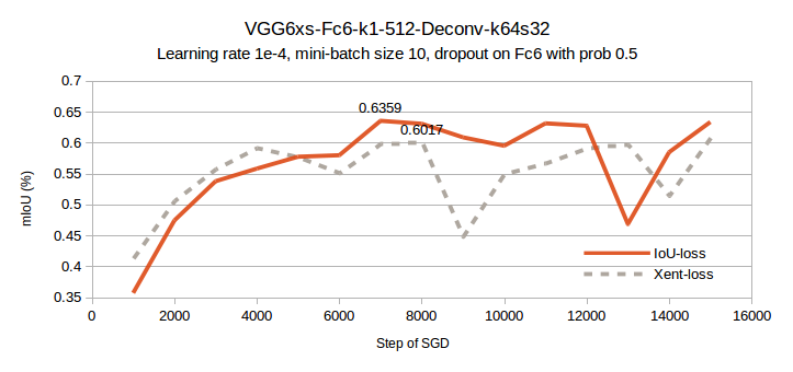
A fairly low capacity model, the VGG6xs-Fc6-k1-512-Deconv-k64s32, was used to do an apples to apples comparison of the two loss functions. This is my own naming convention, but essentially we have: the front end of a VGG16 trimmed down to 5 convolution layers, keeping one of each differently sized layer, number of filters in the first layer reduced from 64 to 16, but still doubling in each subsequent layer, ‘Fc6’ has kernel size 1x1 instead of 7x7, and 512 hiddens, a single deconvolution layer with 64x64 kernel and stride 32.

My dataset has a class distribution of approximately 13% class 1 for (training) and 40% class 1 for (validation). In my very preliminary experiments, I have found the IoU method to be much more sensitive to selection of learning rate and batch size, even with the fairly robust ADAM gradient descent scheme. A fairly high learning rate of 1e-3 led to an unusual instability where the the network always predicted class 0, with a few small point sources of class 1, resulting in a flatline validation mIoU of 31%. This checks out with the aforementioned class balance since we get approx 0% IoU for class 1, and 60% IoU for class 0 by always predicting class 0, which averages to 30%. It can therefore be said that the network has learned something useful for mIoU scores above 30%.

Reducing the learning rate to 1e-4, adding dropout regularization, and increasing mini-batch size to 10, resulted in a fairly nice comparison of the two loss functions. The only difference between the solid and dashed lines in the above figure is that ‘IoU-loss’ was trained with the loss function from Listing 2, while ‘Xent-loss’ was trained with cross-entropy softmax loss as in Listing 1. Optimizing IoU directly resulted in a 3.42% boost in mIoU on my validation set. This difference will likely grow when a higher capacity model is used.

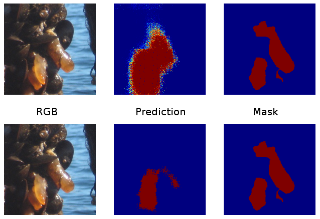
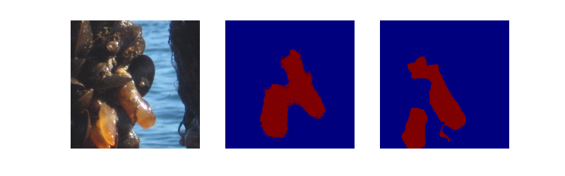
The above image shows from left to right, a sample input, network output at step 5800, and mask. The top uses the IoU loss from Listing 2, while the bottom uses cross-entropy loss from Listing 1. In general, the IoU loss recovers false-negatives but makes more false-positives. The top is fuzzy around the object border because the output has not been thresholded.

Above, IoU loss, below, xent loss.

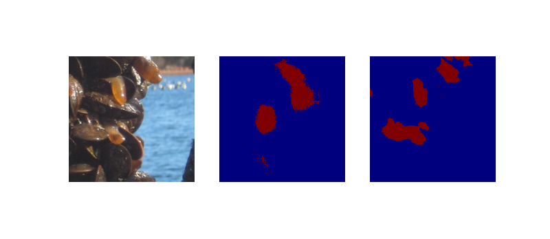
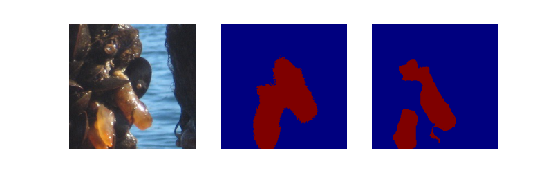
Below are some more samples drawn for validation images, with models trained to 11k steps.

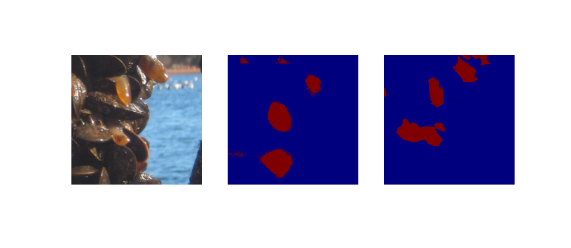
Above, IoU loss gets 3/3 of class 1 objects, while below, xent loss identifies 2/3.